Excel’s VLOOKUP function is a powerful tool for retrieving data from large datasets. It allows you to search for a specific value in one table and return a corresponding value from another table. In this article, we’ll go over how to create a VLOOKUP in Excel step by step.
Step 1: Prepare your data
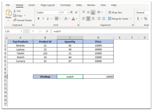
The first step in creating a VLOOKUP is to prepare your data. You will need two tables: one that contains the data you want to search (the lookup table), and another that will receive the returned value (the results table). Make sure your data is organized into columns and that the columns have appropriate headings
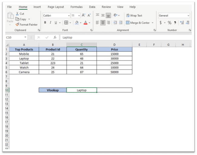
Step 2: Select the cell where you want to display the returned value
Go to the results table and select the cell where you want the returned value to appear. This will be the first argument in the VLOOKUP formula.
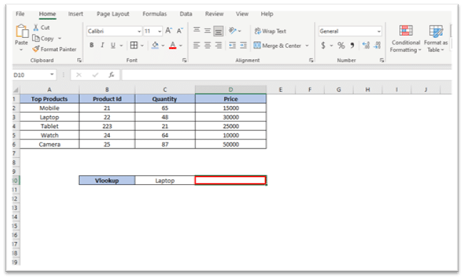
Step 3: Start the formula
Begin the formula by typing “=VLOOKUP(” into the formula bar. This will open the VLOOKUP function and allow you to start entering your arguments.
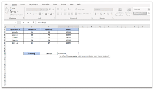
Step 4: Enter the lookup value
The first argument in the VLOOKUP formula is the lookup value. This is the value you want to search for in the lookup table. Enter the lookup value in quotes and close the quotes with a comma.
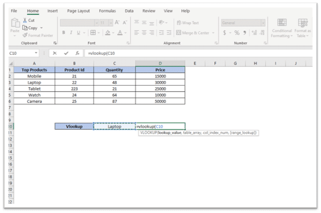
Step 5: Enter the lookup range
The second argument in the VLOOKUP formula is the lookup range. This is the range of cells in the lookup table that contain the data you want to search. Enter the range in the following format: “lookup_table_name[[start_cell]:[end_cell]]”. For example, if your lookup table is named “LookupTable” and starts in cell A1 and ends in cell D6, you would enter “LookupTable[[A1]:[D6]]”.
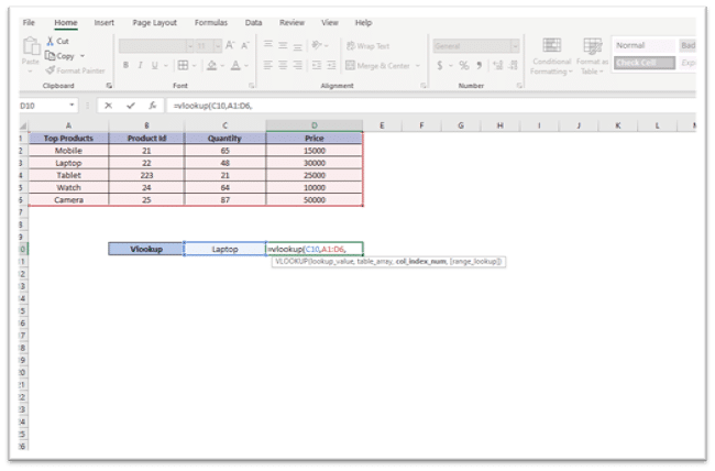
Step 6: Enter the column index number
The third argument in the VLOOKUP formula is the column index number. This is the number of the column in the lookup table that contains the data you want to return. For example, if the data you want to return is in the third column of the lookup table, you would enter “3”.
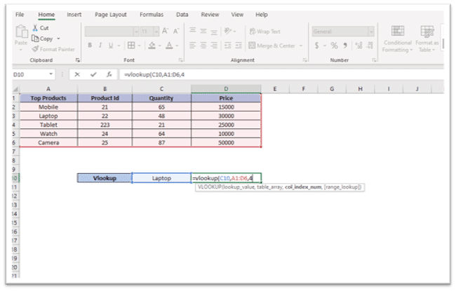
Step 7: Enter the range lookup value
The fourth and optional argument in the VLOOKUP formula is the range lookup value. This is either “TRUE” or “FALSE” and determines whether the VLOOKUP should find an exact match or an approximate match. If you want an exact match, enter “FALSE”. If you want an approximate match, enter “TRUE”. If you omit this argument, Excel will default to “TRUE”.
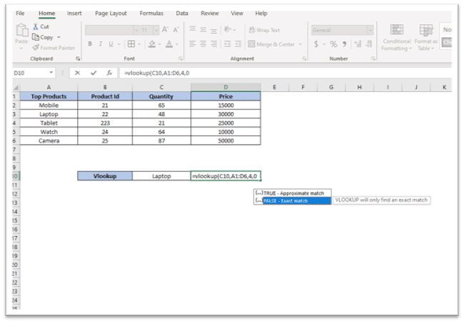
Step 8: Close the formula
Close the formula by typing “)” and press “Enter”. Your VLOOKUP formula should now be complete.
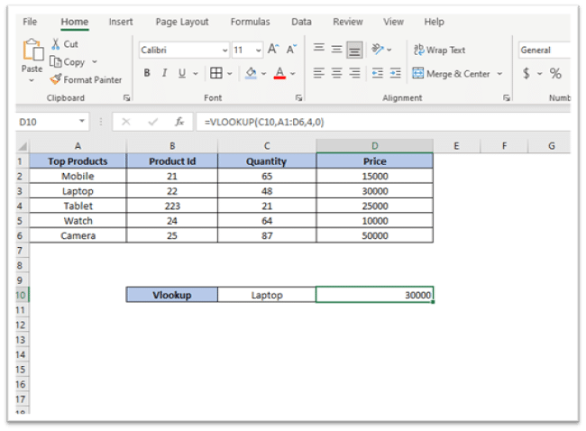
Step 9: Test your VLookup formula in Microsoft Excel
Test your formula by changing the lookup value in the results table to verify that the correct data is returned from the lookup table.
In conclusion, creating a VLOOKUP in Excel is a relatively straightforward process that can greatly increase your efficiency when working with large datasets. With these step by step instructions, you’ll be able to create a VLOOKUP formula in no time. You can find Microsoft office for sale on various online platforms. Many of these platforms also offer Microsoft software downloads, allowing you to easily install the software on your device and start using it right away. Microsoft Office 11 Pro has everything you need to get the job done efficiently and effectively.

