Pivot tables in Excel are a powerful tool for analyzing and summarizing large amounts of data. They allow you to quickly and easily see patterns and trends in your data, making it easier to make informed decisions. In this article, we’ll go over how to create a pivot table in Excel step by step.
Step 1: Prepare your data
The first step in creating a pivot table is to prepare your data. Make sure your data is organized into columns and that the columns have appropriate headings. It’s also a good idea to remove any blank rows or columns from your data.
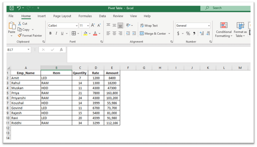
Step 2: Select your data
Select the data that you want to include in your pivot table. This can be a single range of cells or multiple ranges of cells.
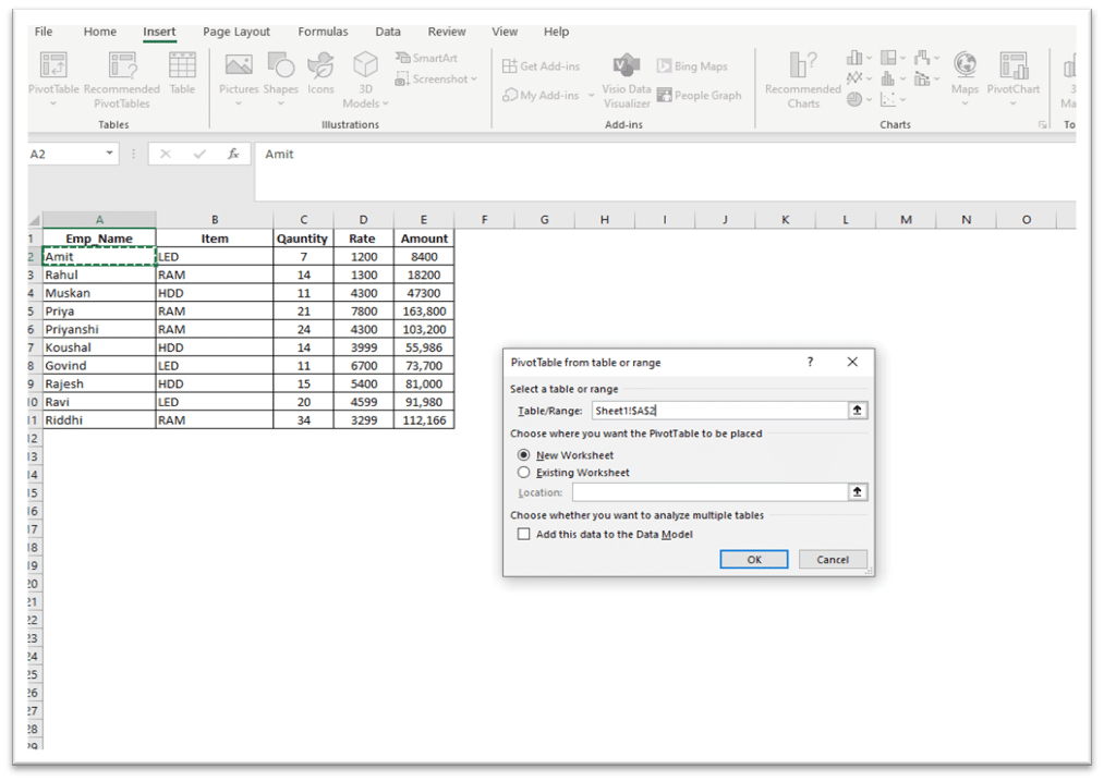
Step 3: Start the pivot table wizard
To start the pivot table wizard, go to the “Insert” tab on the ribbon and select “Pivot Table”. You will be prompted to select the data that you want to include in your pivot table.
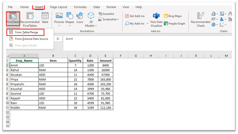
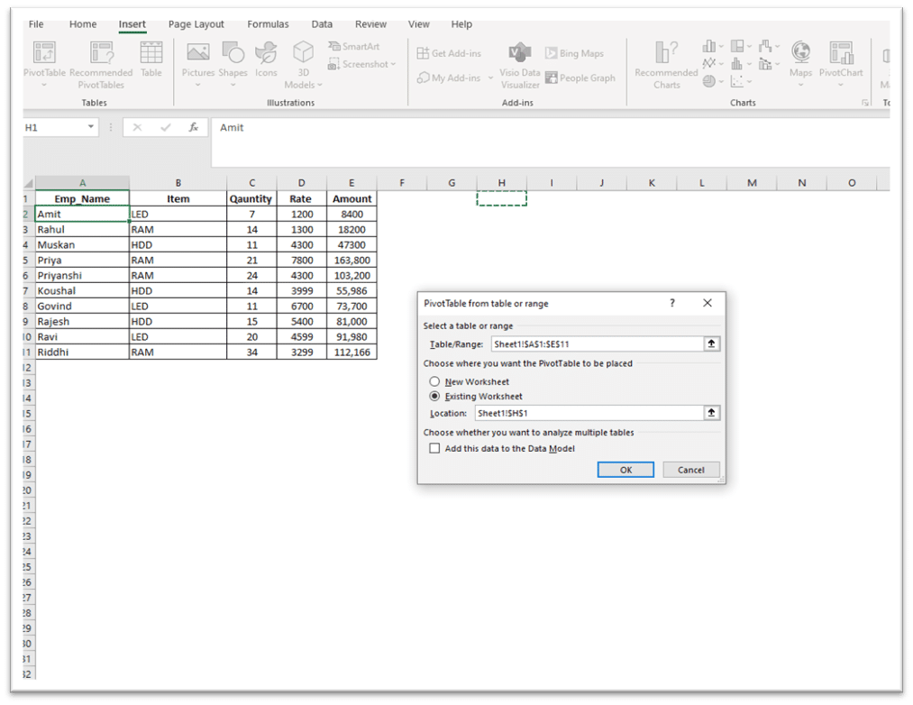
Step 4: Choose the location for your pivot table
Next, choose the location for your pivot table. You can either create a new worksheet for your pivot table or place it in an existing worksheet.
step 5: Select the fields for your pivot table
In the “Pivot Table Fields” pane, select the fields that you want to include in your pivot table. You can add fields to the “Rows”, “Columns”, and “Values” areas. The fields that you add to the “Values” area will become the values that are summarized in your pivot table.
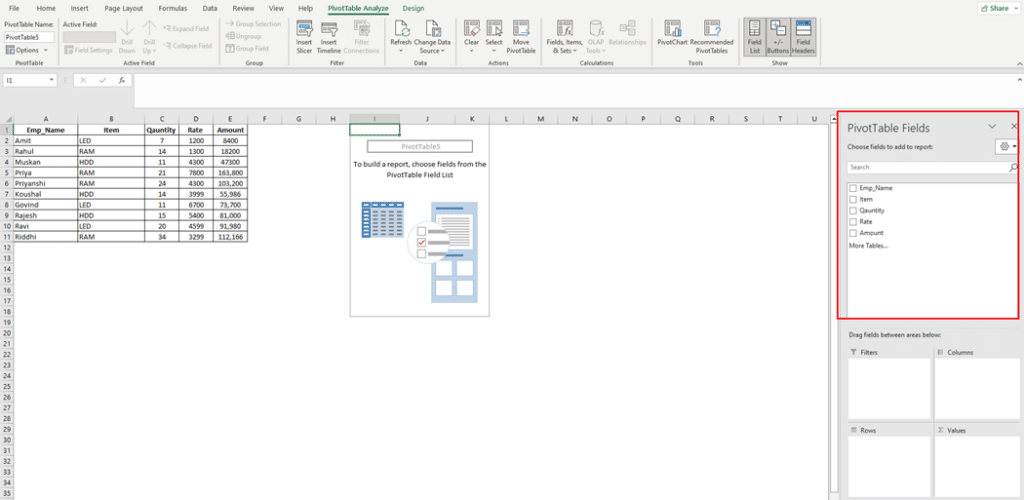
Step 6: Choose the summary calculation
For each field in the “Values” area, you can choose the summary calculation that you want to use. Common summary calculations include “Sum”, “Average”, “Count”, and “Max”.
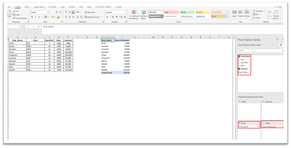
Step 7: Apply any filters or sorting
You can also apply filters or sorting to your pivot table to further refine the data that is displayed. To do this, go to the “Analyze” tab on the ribbon and select “Sort & Filter”.
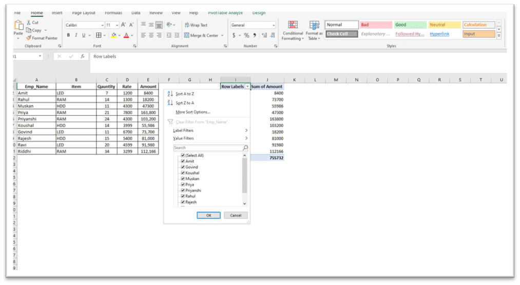
Step 8: Format your pivot table
Finally, you can format your pivot table to make it more readable and visually appealing. You can change the font, font size, and font color, as well as add borders and shading. To format your pivot table, go to the “Design” tab on the ribbon.
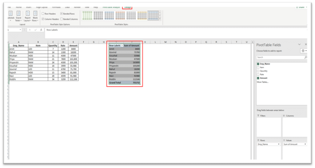
In conclusion, creating a pivot table in Excel is a quick and easy way to analyze and summarize large amounts of data. With these step by step instructions, you’ll be able to create a pivot table in no time. In windows 11 Pro you can made pivot table as this have a good updates in office software programs.

